In this tutorial you will try to reproduce one of the figures in Shapiro et al.. To see which one, execute the second code block below.
Reference: High-Resolution Surface-Wave Tomography from Ambient Seismic Noise, Nikolai M. Shapiro, et al. Science 307, 1615 (2005); DOI: 10.1126/science.1108339
Authors:
- Celine Hadziioannou
- Ashim Rijal
# Configuration step (Please run it before the code!)

import numpy as np
import sys, obspy, os
import matplotlib.pyplot as plt

from obspy.core import UTCDateTime
from obspy.clients.fdsn import Client
from obspy.geodetics import gps2dist_azimuth as gps2DistAzimuth # depends on obspy version; this is for v1.1.0
#from obspy.core.util import gps2DistAzimuth

#from PIL import Image
import requests
from io import BytesIO

%matplotlib inline
import warnings
warnings.filterwarnings('ignore')
In this notebook
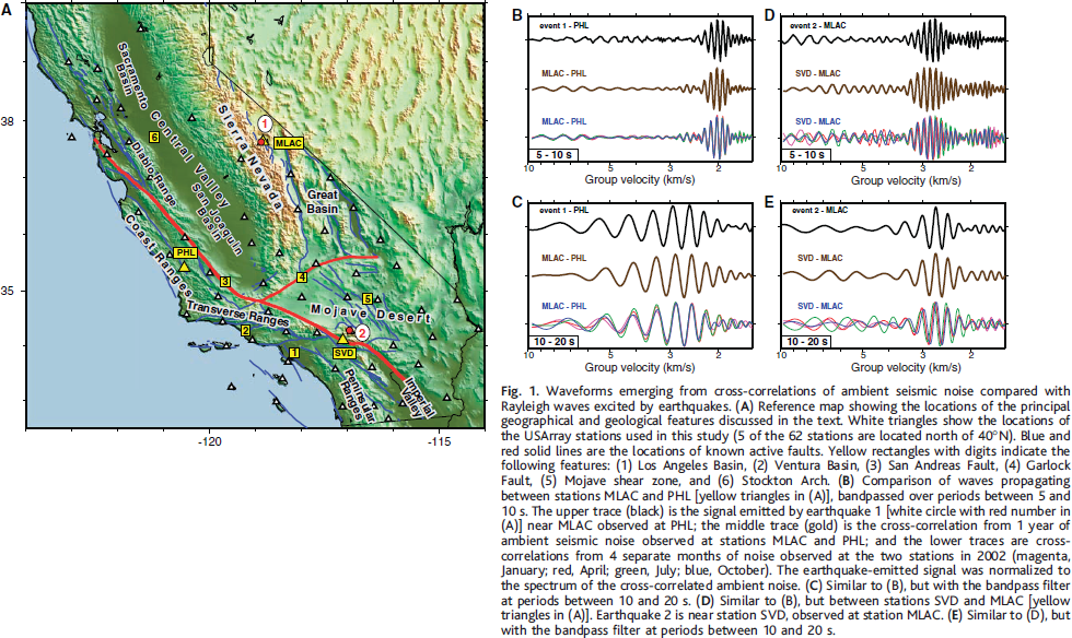
We will reproduce figure B below. This figure compares: 1) the seismogram from an event near station MLAC, recorded at station PHL (top) 2) the "Greens function" obtained by correlating noise recorded at stations MLAC and PHL (center and bottom)
All bandpassed for periods between 5 - 10 seconds.
1. Read in noise data
Read the noise data for station MLAC into a stream.
Then, read in noise data for station PHL. Add this to the stream created above.
These two data files contain 90 days of vertical component noise for each station.
If you need data for more than 90 days, it can be downloaded form IRIS database.
# Shapiro et al. use noise data from MLAC and PHL stations

num_of_days = 90                            # no of days of data: change if more than 90days of data is required
if num_of_days <= 90:
    # get noise data for station MLAC
    stn = obspy.read('https://raw.github.com/ashimrijal/NoiseCorrelation/master/data/noise.CI.MLAC.LHZ.2004.294.2005.017.mseed')
    # get noise data for the station PHL and add it to the previous stream
    stn += obspy.read('https://raw.github.com/ashimrijal/NoiseCorrelation/master/data/noise.CI.PHL.LHZ.2004.294.2005.017.mseed')
    # if you have data stored locally, comment the stn = and stn += lines above
    # then uncomment the following 3 lines and adapt the path:
    # stn = obspy.read('./noise.CI.MLAC.LHZ.2004.294.2005.017.mseed')
    # stn += obspy.read('noise.CI.PHL.LHZ.2004.294.2005.017.mseed')
    # ste = obspy.read('event.CI.PHL.LHZ.1998.196.1998.196.mseed')
else:
    # download data from IRIS database
    client = Client("IRIS")                               # client specification
    t1 = UTCDateTime("2004-10-20T00:00:00.230799Z")       # start UTC date/time
    t2 = t1+(num_of_days*86400)                           # end UTC date/time
    stn = client.get_waveforms(network="CI", station="MLAC",location="*", channel="*",
                               starttime=t1, endtime=t2)  # get data for MLAC
    stn += client.get_waveforms(network="CI", station="PHL", location="*", channel="*",
                                starttime=t1, endtime=t2) # get data for PHL and add it to the previous stream
2. Preprocess noise
Preprocessing 1
Just to be sure to keep a 'clean' original stream, first copy the noise stream with st.copy() The copied stream is the stream you will use from now on.
In order to test the preprocessing without taking too long, it's also useful to first trim this copied noise data stream to just one or a few days. This can be done with st.trim(), after defining your start- and endtime.
Many processing functionalities are included in Obspy. For example, you can remove any (linear) trends with st.detrend(), and taper the edges with st.taper(). Different types of filter are also available in st.filter().
- first detrend the data.
- next, apply a bandpass filter to select the frequencies with most noise energy. The secondary microseismic peak is roughly between 0.1 and 0.2 Hz. The primary microseismic peak between 0.05 and 0.1 Hz. Make sure to use a zero phase filter! (specify argument zerophase=True)
# Preprocessing 1

stp = stn.copy()                                                 # copy stream
t = stp[0].stats.starttime
stp.trim(t, t + 4 * 86400)                                       # shorten stream for quicker processing

stp.detrend('linear')                                            # remove trends using detrend
stp.taper(max_percentage=0.05, type='cosine')                    # taper the edges
stp.filter('bandpass', freqmin=0.1, freqmax=0.2, zerophase=True) # filter data of all traces in the streams
Preprocessing 2
Some additional useful processing functions are provided in the following cell named Functions
- For each trace in the stream, apply spectral whitening on the frequency range you chose before (either [0.1 0.2]Hz or [0.05 0.1]Hz), using function
whiten.
For the time normalization, the simplest option is to use the one-bit normalization option provided in function
normalize.Optional: play around with different normalization options, such as clipping to a certain number of standard deviations, or using the running absolute mean normalization.
A brief desription of individual functions (see the next cell) are as follows:
1) whiten:
    spectral whitening of trace `tr` using a cosine tapered boxcar between `freqmin` and `freqmax`
    (courtesy Gaia Soldati & Licia Faenza, INGV)
2) correlateNoise:
    correlate two stations, using slices of 'corrwin' seconds at a time correlations are also stacked.
    NB hardcoded: correlates 1st with 2nd station in the stream only signals are merged - any data gaps are
    filled with zeros.
    st : stream containing data from the two stations to correlate
    stations : list of stations
    corrwin : correlation window length
    returns 'corr' (all correlations) and 'stack' (averaged correlations)
3) plotStack:
    plots stack of correlations with correct time axis
    st: stream containing noise (and station information)
    stack: array containing stack
    maxlag: maximum length of correlation to plot (in seconds)
4) plotXcorrEvent:
    plot the noise correlation (MLAC, PHL) alongside the 1998 event signal
    st : event stream
    stn : noise stream
    stack : noise correlation array
    maxlag : maximum length of correlation, in seconds
    acausal : set to True to use acausal part (=negative times) of the correlation
    figurename : if a filename is specified, figure is saved in pdf format
5) Normalize:
    Temporal normalization of the traces, most after Bensen 2007. NB. before this treatment, traces must be
    demeaned, detrended and filtered. Description of argument:

    norm_method="clipping"
        signal is clipped to 'clip_factor' times the std
        clip_factor recommended: 1 (times std)

    norm_method="clipping_iter"
        the signal is clipped iteratively: values above 'clip_factor * std'
        are divided by 'clip_weight'. until the whole signal is below
        'clip_factor * std'
        clip_factor recommended: 6 (times std)


    norm_method="ramn"
        running absolute mean normalization: a sliding window runs along the
        signal. The values within the window are used to calculate a
        weighting factor, and the center of the window is scaled by this
        factor.
            weight factor: w = np.mean(np.abs(tr.data[win]))/(2. * norm_win + 1)
        finally, the signal is tapered with a tukey window (alpha = 0.2).

        norm_win: running window length, in seconds.
          recommended: half the longest period

    norm_method="1bit"
        only the sign of the signal is conserved
6) get_window:
    Return tukey window of length N
    N: length of window
    alpha: alpha parameter in case of tukey window.
    0 -> rectangular window
    1 -> cosine taper
    returns: window (np.array)
Doc of scipy.signal.get_window
# Functions
# collection of functions used in noise correlation processing

def normalize(tr, clip_factor=6, clip_weight=10, norm_win=None, norm_method="1bit"):

    if norm_method == 'clipping':
        lim = clip_factor * np.std(tr.data)
        tr.data[tr.data > lim] = lim
        tr.data[tr.data < -lim] = -lim

    elif norm_method == "clipping_iter":
        lim = clip_factor * np.std(np.abs(tr.data))

        # as long as still values left above the waterlevel, clip_weight
        while tr.data[np.abs(tr.data) > lim] != []:
            tr.data[tr.data > lim] /= clip_weight
            tr.data[tr.data < -lim] /= clip_weight

    elif norm_method == 'ramn':
        lwin = tr.stats.sampling_rate * norm_win
        st = 0                                               # starting point
        N = lwin                                             # ending point

        while N < tr.stats.npts:
            win = tr.data[st:N]

            w = np.mean(np.abs(win)) / (2. * lwin + 1)

            # weight center of window
            tr.data[st + lwin / 2] /= w

            # shift window
            st += 1
            N += 1

        # taper edges
        taper = get_window(tr.stats.npts)
        tr.data *= taper

    elif norm_method == "1bit":
        tr.data = np.sign(tr.data)
        tr.data = np.float32(tr.data)

    return tr


def get_window(N, alpha=0.2):

    window = np.ones(N)
    x = np.linspace(-1., 1., N)
    ind1 = (abs(x) > 1 - alpha) * (x < 0)
    ind2 = (abs(x) > 1 - alpha) * (x > 0)
    window[ind1] = 0.5 * (1 - np.cos(np.pi * (x[ind1] + 1) / alpha))
    window[ind2] = 0.5 * (1 - np.cos(np.pi * (x[ind2] - 1) / alpha))
    return window


def whiten(tr, freqmin, freqmax):

    nsamp = tr.stats.sampling_rate

    n = len(tr.data)
    if n == 1:
        return tr
    else:
        frange = float(freqmax) - float(freqmin)
        nsmo = int(np.fix(min(0.01, 0.5 * (frange)) * float(n) / nsamp))
        f = np.arange(n) * nsamp / (n - 1.)
        JJ = ((f > float(freqmin)) & (f<float(freqmax))).nonzero()[0]

        # signal FFT
        FFTs = np.fft.fft(tr.data)
        FFTsW = np.zeros(n) + 1j * np.zeros(n)

        # Apodization to the left with cos^2 (to smooth the discontinuities)
        smo1 = (np.cos(np.linspace(np.pi / 2, np.pi, nsmo+1))**2)
        FFTsW[JJ[0]:JJ[0]+nsmo+1] = smo1 * np.exp(1j * np.angle(FFTs[JJ[0]:JJ[0]+nsmo+1]))

        # boxcar
        FFTsW[JJ[0]+nsmo+1:JJ[-1]-nsmo] = np.ones(len(JJ) - 2 * (nsmo+1))\
        * np.exp(1j * np.angle(FFTs[JJ[0]+nsmo+1:JJ[-1]-nsmo]))

        # Apodization to the right with cos^2 (to smooth the discontinuities)
        smo2 = (np.cos(np.linspace(0., np.pi/2., nsmo+1.))**2.)
        espo = np.exp(1j * np.angle(FFTs[JJ[-1]-nsmo:JJ[-1]+1]))
        FFTsW[JJ[-1]-nsmo:JJ[-1]+1] = smo2 * espo

        whitedata = 2. * np.fft.ifft(FFTsW).real

        tr.data = np.require(whitedata, dtype="float32")

        return tr


def correlateNoise(st, stations, corrwin):

    print ('correlating stations', (stations[0], stations[1]))

    # initialize sliding timewindow (length = corrwin) for correlation
    # start 1 corrwin after the start to account for different stream lengths
    timewin = st.select(station=stations[1])[0].stats.starttime + corrwin

    # loop over timewindows
    # stop 1 corrwin before the end to account for different stream lengths
    while timewin < st.select(station=stations[0])[-1].stats.endtime - 2*corrwin:
        sig1 = st.select(station=stations[0]).slice(timewin, timewin+corrwin)
        sig1.merge(method=0, fill_value=0)
        sig2 = st.select(station=stations[1]).slice(timewin, timewin+corrwin)
        sig2.merge(method=0, fill_value=0)
        xcorr = np.correlate(sig1[0].data, sig2[0].data, 'same')

        try:
            # build array with all correlations
            corr = np.vstack((corr, xcorr))
        except:
            # if corr doesn't exist yet
            corr = xcorr

        # shift timewindow by one correlation window length
        timewin += corrwin

        # stack the correlations; normalize
        stack = np.sum(corr, 0)
        stack = stack / float((np.abs(stack).max()))
    print ("...done")

    return corr, stack


def plotStack(st, stack, maxlag, figurename=None):

    # define the time vector for the correlation (length of corr = corrwin + 1)
    limit = (len(stack) / 2.) * st[0].stats.delta
    timevec = np.arange(-limit, limit, st[0].stats.delta)

    plt.plot(timevec, stack, 'k')
    stations = list(set([_i.stats.station for _i in st]))
    plt.title("Stacked correlation between %s and %s" % (stations[0], stations[1]))
    plt.xlim(-maxlag, maxlag)
    plt.xlabel('time [s]')

    if figurename is not None:
        fig.savefig(figurename, format="pdf")
    else:
        plt.show()


def plotXcorrEvent(st, stn, stack, maxlag, acausal=False, figurename=None):

    eventtime = UTCDateTime(1998,7,15,4,53,21,0)                 # event near MLAC

    # station locations
    latP, lonP = 35.41, -120.55                                  # station PHL
    latM, lonM = 37.63, -118.84                                  # station MLAC
    latE, lonE = 37.55, -118.809                                 # event 1998

    # calculate distance between stations
    dist = gps2DistAzimuth(latP, lonP, latM, lonM)[0]            # between PHL and MLAC
    distE = gps2DistAzimuth(latP, lonP, latE, lonE)[0]           # between event and PHL
                                                                 #
    # CROSSCORRELATION
    # reverse stack to plot acausal part (= negative times of correlation)
    if acausal:
        stack = stack[::-1]

    # find center of stack
    c = int(np.ceil(len(stack)/2.) + 1)

    #cut stack to maxlag
    stack = stack[c - maxlag * int(np.ceil(stn[0].stats.sampling_rate)) : c + maxlag * int(np.ceil(stn[0].stats.sampling_rate))]

    # find new center of stack
    c2 = int(np.ceil(len(stack)/2.) + 1)

    # define time vector for cross correlation
    limit = (len(stack) / 2.) * stn[0].stats.delta
    timevec = np.arange(-limit, limit, stn[0].stats.delta)
    # define timevector: dist / t
    timevecDist = dist / timevec

    # EVENT
    ste = st.copy()
    st_PHL_e = ste.select(station='PHL')

    # cut down event trace to 'maxlag' seconds
    dt = len(stack[c2:])/stn[0].stats.sampling_rate                  #xcorrlength
    st_PHL_e[0].trim(eventtime, eventtime + dt)

    # create time vector for event signal
    # extreme values:
    limit = st_PHL_e[0].stats.npts * st_PHL_e[0].stats.delta
    timevecSig = np.arange(0, limit, st_PHL_e[0].stats.delta)

    # PLOTTING
    fig = plt.figure(figsize=(12.0, 6.0))
    ax1 = fig.add_subplot(2,1,1)
    ax2 = fig.add_subplot(2,1,2)

    # plot noise correlation
    ax1.plot(timevecDist[c2:], stack[c2:], 'k')
    ax1.set_title('Noise correlation between MLAC and PHL')

    # plot event near MLAC measured at PHL
    ax2.plot(distE/timevecSig, st_PHL_e[0].data / np.max(np.abs(st_PHL_e[0].data)), 'r')
    ax2.set_title('Event near MLAC observed at PHL')

    ax2.set_xlim((0, 8000))
    ax1.set_xlim((0, 8000))

    ax2.set_xlabel("group velocity [m/s]")

    if figurename is not None:
        fig.savefig(figurename, format="pdf")
    else:
        plt.show()
Actual preprocessing happens here -- this can take a while!
# Preprocessing 2
st = stp.copy()                            # copy stream

for tr in st:
    tr = normalize(tr, norm_method="1bit")
    tr = whiten(tr, 0.1, 0.2)
print ('done!')
Cross-correlation
Once you're happy with the preprocessing, you can calculate the cross-correlation using correlateNoise function. The cross-correlation are computed by slices of a few hours each (specified in corrwin).
For correlateNoise function
- input: stream, list of stations (here: ['MLAC', 'PHL']), slice length in seconds
- output: all individual correlations, stack
# Cross-correlate
xcorr, stack = correlateNoise(st, ['MLAC','PHL'], 7200)
The resulting stack can be plotted with plotStack function. Since it doesn't make much sense to look at a 2 hour long correlation signal, you can decide to plot only the central part by specifying a maxlag (in seconds).
# Plotting

plotStack(st,stack,400)

If you're only working with a few days of noise (after trimming), this plot probably doesn't look very nice. You could go back to the code block named 'preprocessing 1', and keep a longer noise record (10 days works quite well already).
Compare to event trace
In 1998, a M = 5.1 event occurred next to station MLAC. This event was recorded at PHL and we read this data.
- read the event data to a separate stream
ste = obspy.read('https://raw.github.com/ashimrijal/NoiseCorrelation/master/data/event.CI.PHL.LHZ.1998.196.1998.196.mseed')
# if data is stored locally, uncomment the following line and comment the line above:
#ste = obspy.read('./event.CI.PHL.LHZ.1998.196.1998.196.mseed')
Preprocess event
The event signal should be processed in a similar way to the noise.
- detrend in the same way as before
- bandpass filter for the same frequencies as chosen above
- apply spectral whitening to each trace in the event stream to ensure the spectrum is comparable to the noise.
# Preprocessing

ste.detrend('linear')
ste.filter('bandpass', freqmin=0.1, freqmax=0.2, zerophase=True)
for tr in ste:
    tr = whiten(tr, 0.1, 0.2)
Plot!
A plotting function is provided to plot both signals alongside: plotXcorrEvent.
- input: event stream, noise stream, stack, maxlag
# Plotting

plotXcorrEvent(ste, stn, stack, 400)
